.BSc - Niklas Kopp

A novel method for high-performance mass spectometry (MS1) sample classification using pattern recognition and deep learning

A superficial technical summary of my Bachelors Thesis.

Disclaimer
As provided, I do not claim full correctness or completeness of the content.
While the bibliography is complete, some contents are skipped, and citations may be imperfect due to the summarization process (including AI assistance).
All code is presented in pseudocode for readability, and table and figure captions were not reworked.

LC-MS

LC-MS combines liquid chromatography to separate peptides and mass spectrometry to identify them.

Pattern Recognition

Pattern recognition algorithms are computational methods that detect and classify structured patterns in data.

Deep Learning

Deep learning uses multi-layer neural networks to learn complex patterns from data.

Abstract

This bachelor’s thesis presents a novel approach for analyzing mass spectrometry (MS) data by combining pattern-based abstraction with convolutional neural networks (CNNs).

Mass spectrometry is a multi-step process that involves sample preparation, ionization, and detection to determine the mass-to-charge ratio and abundance of molecules in complex biological samples. The resulting data are highly complex and large in size, containing overlapping signals from diverse sources, including biological components, reagents, instrumental noise, and resolution artifacts. Accurate interpretation therefore requires careful signal deconvolution, noise reduction, and contaminant detection.

Motivated by the growing relevance of proteomics—especially following the COVID-19 pandemic—this work aims to improve the efficiency and accuracy of MS data analysis. Unlike existing deep learning approaches that primarily focus on peptide identification and prediction, this thesis targets the earlier MS1 stage to identify features of interest and to accelerate the assignment of signals to their procedural origin.

After reviewing established methods in MS-based proteomics, the thesis introduces relevant concepts in molecular biology, proteomics, and deep learning. It then presents four novel techniques: two denoising algorithms to enhance MS data for pattern recognition, a CNN-based image classification model for assigning detected features to classes, and a blueprint for a new alignment algorithm to correct data deviations not well handled by current methods.

The proposed framework aims to enable more reliable classification of medical samples across hierarchical label groups, reduce the impact of manual labelling errors, and highlight biologically relevant markers for further investigation.

Introduction

This thesis provides a comprehensive process analysis for mass spectrometry (MS)-based proteomics in the context of pattern recognition and deep learning techniques. Its primary objective is to introduce a novel method that combines deep learning, visual abstraction of MS data, and pattern recognition algorithms to enable fast sample classification and anomaly detection in proteomics raw data based on the precursor ion scan, referred to as “MS1” throughout this thesis [1]. By leveraging the interconnectedness of molecular features arising from highly correlated biochemical processes, this method enhances the interpretation and analysis of complex samples and opens new avenues to link features detected by bottom-up mass spectrometry [1]. The approach aims to classify samples of medical origin across multiple hierarchical label groups, reduce the impact of manual labelling errors by verifying sample origin, and highlight biological markers and other features of interest for further analysis. Additionally, by introducing image-based representations of MS data, both storage requirements and computational costs can be substantially reduced.

To understand this approach, it is essential to establish foundational knowledge of molecular biology, proteomics, and mass spectrometry. Furthermore, a basic understanding of artificial neural networks and the underlying mathematical principles is required. By providing a comprehensive outline that encompasses these areas, this thesis equips the reader with the background necessary to understand the connections and design decisions made within this research.

The Previous Work chapter summarizes the most significant state-of-the-art methods evaluated prior to developing the concepts presented here. During the preparation of this thesis, nine deep learning models from diverse scientific fields were assessed for their applicability to the defined classification goals, including two undisclosed models. These fields included Medical Imaging, General Image Classification, and Deep Learning approaches for Mass Spectrometry [2–8]. In addition, ten clustering and MS data alignment approaches were implemented and evaluated to determine their suitability for identifying reliable patterns and preserving data integrity during pattern alignment [9–14].

The Background chapter first introduces fundamental concepts of molecular biology and proteomics. It then outlines the preparation steps required to process biological samples for use in MS experiments, illustrated with a human blood sample as an example.

The second subchapter examines an exemplary data-independent acquisition (DIA) mass spectrometry experiment on the processed sample, emphasizing the complexity of the resulting data and selected analysis methods. This analysis provides the basis for identifying reliable patterns while highlighting potential limitations and additional signals introduced by the applied methods.

Finally, the third subchapter explains convolutional neural networks (CNNs) and introduces fundamental deep learning terminology that will be referenced in the subsequent main chapters.

Summary - Previous Work / Background

Deep Learning

DLearnMS [7] is a deep learning framework for biomarker detection in LC-MS proteomics data. It tackles high dimensionality, low sample size, and limited interpretability using convolutional neural networks (CNNs) combined with layer-wise relevance propagation to identify biomarkers. It outperforms conventional methods by reducing false positives while maintaining true positives and shows that overly complex architectures (e.g. ResNet32) can cause overfitting and long runtimes. It builds on Iravani et al. [6], who proposed using image-based data transformation and a 10-layer DNN for feature selection and classification. Together, these works motivated the use of simpler CNN architectures in this thesis to avoid overfitting, reduce runtime, and improve interpretability. They also highlight the role of saliency maps, stride size, and kernel choice on performance [15].

MSTranc [5] investigates applying pretrained image classification models to raw MS data, resizing MS images to 224×224 and feeding them to standard CNN encoders. It validates that MS images are suitable for signal classification, but notes two drawbacks: resolution loss from resizing and reliance on predefined small input dimensions. Its repository provides tools for converting raw MS data into tensors suitable for deep models [16].

MSpectraAI [4] is an open-source platform that applies deep neural networks (DNNs) to large-scale MS1 proteomics data. It uses an m/z window-based normalization strategy and matrix-form inputs to achieve high accuracy on multi-tumor datasets (available on GitHub [17]). While its normalization approach is debated, the work reinforces the assumption that stable signal patterns exist between normal and cancer samples, which underpins this thesis. Unlike MSpectraAI’s matrix focus, this thesis applies CNNs to image-based abstractions of MS data, where padding [18] and convolutional kernels [19] inherently handle signal range and abundance variations.

Pattern Recognition and Alignment

Self-Organizing Maps (SOM) [9, 10] use unsupervised competitive learning to produce low-dimensional feature maps. They contribute the idea of anchor points and relational grids that can dynamically adapt previously observed feature maps to new inputs, complementing CNN-based approaches.

Dynamic Time Warping (DTW) [11, 20] aligns time series by stretching or compressing local segments. It inspired this thesis’s use of curve-based signal abstraction for LC gradient cutoffs. However, it showed weaknesses in preserving coordinates of high-intensity peaks, especially with varying signal intensities.

MS1Connect [12, 21] measures similarities between MS1 runs via a maximum bipartite matching approach, showing strong correlation with MS2-based similarity scores. It contributed benchmark values for alignment runtime and accuracy, but also confirmed that high-intensity peak positions are often not preserved, as seen with DTW. Its openly available code makes it a viable fallback.

OpenMS MapAlignerPoseClustering [22–25] aligns retention times via a star-like progressive alignment with a superposition–consensus framework. It provided the initial concept for a star-wise alignment strategy used in this thesis. However, its consensus-based approach tended to neglect high-intensity patterns (anchor points). Still, its robust OpenMS integration, documentation, and community support proved very helpful during development.

Background

Molecular Biology and Proteomics

Central Dogma of Molecular Biology

The central dogma captures the directional flow of genetic information from DNA to RNA to protein. In standard transcription, one DNA strand serves as the template to synthesize mRNA, which in eukaryotes is processed in the nucleus before translation in the cytosol. Translation converts mRNA codons—triplets of nucleotides—into amino acids with the help of tRNAs and ribosomes. While the code is degenerate, with several codons mapping to a single amino acid, each codon specifies only one amino acid, keeping translation unambiguous. Viral exceptions exist, using RNA-dependent RNA or RNA-dependent DNA polymerases. [26, 27]

Proteomics

Proteomics investigates the proteome—the full protein complement of a system—covering structure, function, interactions, and post-translational modifications. Clinical specimens such as blood, urine, or tissue support diagnosis, prognosis, personalized therapy, and biomarker discovery by linking protein patterns to biological states. [27, 28]

Biological Samples

Human blood exemplifies a practical matrix for LC–MS proteomics. Venipuncture enables collection, followed by centrifugation to isolate plasma, which constitutes roughly 55% of blood and contains water, abundant proteins (e.g., albumin), hormones, metabolites, and other solutes. Sample preparation typically includes protein extraction, enzymatic digestion—commonly with trypsin—peptide cleanup, and optional labeling. Missed cleavages and preparation artifacts introduce variability, while salts, detergents, and labels can add contaminants or shift isotope abundances. [27, 29, 30, 31, 32, 33, 34]

Mass Spectrometry

Mass spectrometry (MS) measures mass-to-charge ratios and signal abundances, enabling identification and characterization of biomolecules across diverse fields including proteomics and metabolomics. Continuous advances—from early analyzers to hybrid instruments—have expanded sensitivity, resolution, and throughput, culminating in analyses of highly complex entities such as intact viruses. The COVID-19 era underscored MS as a diagnostic and discovery tool, with community efforts accelerating biomarker identification for disease severity and long-term effects. [1, 28, 35, 36, 37, 38]

Mass Spectrometry Experiment

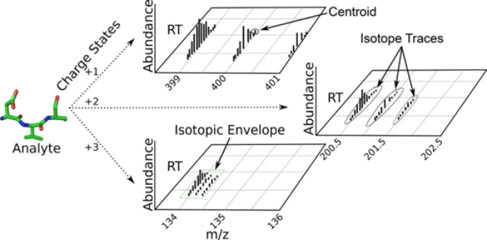
Analyte signals reflect isotopic composition, charge states and adducts, and potential post-translational modifications, alongside retention time when LC is coupled. Together these dimensions produce isotopic envelopes that encode composition and abundance over time. Biological variability and analytical interferences from reagents or contaminants complicate reproducibility, while snapshot limitations and method choices further affect outcomes. LC separation is frequently employed to manage complex matrices such as plasma. [1, 27, 30, 31, 32, 39, 40, 41, 42]

Mass-Spectra

Raw output of the LC-MS

Figure 1 Signals detected from a LC-Mass Spectrometer for a specific analyte. The left diagram illustrates the Isotopic Envelope as characterization of the analyte’s different isotopic variants, separated through time of detection and abundance of detection. Remaining diagrams specify the nomenclature of further frameable contents of the Isotopic Envelope. [41]

Read more

Liquid Chromatography

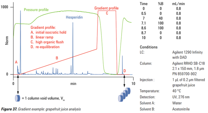
Liquid chromatography couples a mobile solvent mixture with a stationary phase to separate peptides according to physicochemical properties such as polarity, size, or charge. UHPLC, HPLC, and conventional LC differ in particle size, pressure, resolution, and runtime. Real-world variability arises from solvent composition, column aging, carryover, and environmental factors like temperature. Typical runs include an initial isocratic hold, a linear gradient, and a high-organic flush; LC is often interfaced directly to ion sources such as ESI for seamless transfer to MS. [27, 43, 44, 45]

Gradient separation

Visual from LC-MS Software

Figure 2 Gradient separation of grapefruit juice in a LC-Experiment. Illustrated are the different states of an LC-Experiment in relation to an Agilent Technologies separation column. Solvents used for the mobile Phase are Water and Acetonitrile at 40 °C device temperature. The shown peak of Hesperidin refers to the main flavonoid of lemon and orange fruit skin, rendering a highly abundant and specific analyte for orange juice analysis. [44, 45]

Read more

Electrospray Ionization

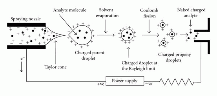
Electrospray ionization (ESI) converts liquid-phase analytes into gas-phase ions, often producing multiple charges for large biomolecules. Ionization efficiency and charge states depend on concentration, emitter geometry, vacuum conditions, and contaminants; adduct formation and ion–molecule reactions further shape observed spectra. [1, 46]

Electrospray Ionization

Schematic

Figure 3 A schematic of the electrospray Ionization process. It shows how the solution is eluted from the emitter tip from the left, which consequently form droplets and results in taylor cone formed upon release, while opposing voltages are applied to both sides. The solvent then further evaporates and forms smaller droplets until charged molecules desorb from the droplets surface and subsequently enter the mass spectrometer on the right side of the schematic. [46]

Read more

Focusing on MS1 in data-independent acquisition, an LTQ Orbitrap architecture serves as the reference. Ions enter under high vacuum and traverse components that can filter, guide, and manipulate beams; for MS1 emphasis, intact precursors are transferred directly to the analyzer, with later normalization accommodating instrument-specific effects. [28, 47, 48]

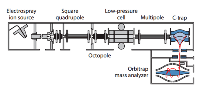
LTQ Orbitrap Mass Spectrometer

A traditional MS Architecture

Figure 4 Schematic of a LTQ Orbitrap Mass spectrometer. It illustrates the traditional LTQ Orbitrap mass spectrometer architecture and scan execution scheme, involving an ion trap and Orbitrap mass analyzer. [47]

Read more

Filter, Guides and Ion Manipulation

Ion optics between source and analyzer provide optional mass filtering, beam focusing, and transmission, and can prepare ions for fragmentation in DDA or DIA. For the MS1-centric view adopted here, the priority is stable precursor transfer; correlations in m/z are preserved, while intensity may require normalization due to device settings or procedural artifacts. [1, 28, 47, 48]

Mass Detection

Mass analyzers separate ions by different physical principles; trapping versus continuous analyzers yield distinct signal characteristics. In the Orbitrap, periodic injection of ion packets leads to oscillatory motion whose image current is recorded and Fourier-transformed to produce high-resolution mass spectra. [1, 28, 48]

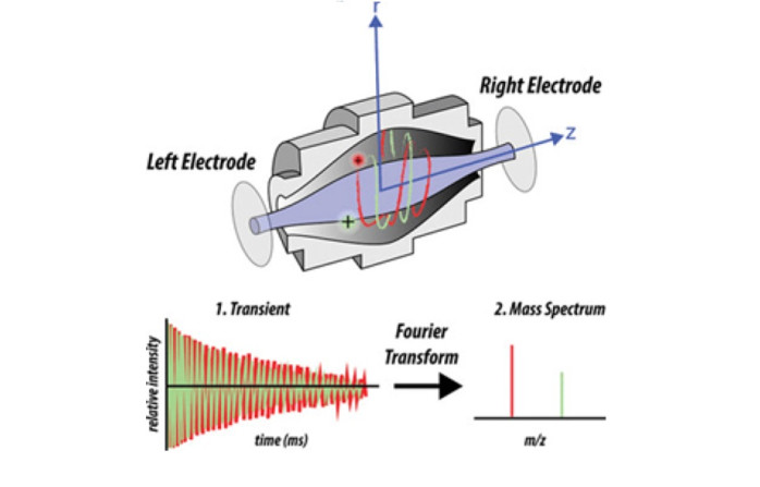
Orbitrap Mass Analyzer

How analytes are measured

Figure 5 Schematic of the Orbitrap FT mass analyzer. The schematic shows a more detailed view for the scan execution which results in a mass spectrum. FT stands for Fourier Transformation and relates to the frequency of ion oscillation in the Orbitrap which are subsequently transformed into signal peaks to yield a mass spectrum. [48]

Read more

Data Handling

Vendors provide instrument control and proprietary formats (e.g., RAW), yet metadata completeness and standardization can vary across makers and runs. Open-source tools such as MaxQuant and Skyline exist, while this work centers on OpenMS for processing and visualization, including TOPPView for interactive inspection. [49, 50, 51, 52, 53, 54]

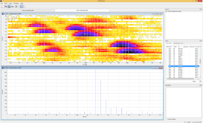
Data visualisation

by OpenMS

Figure 6 TOPPView graphical application for viewing mass spectra and analysis results. TOPPView is a tool to view and analyse all aspects of a measured spectra based on a visual access window on the top. Signals are colored according to the raw peak intensities. On the bottom is a display of an extracted scan from the peak map, identifiable by the vertical dotted line. In the right window every spectra can be accessed directly. [54]

Read more

Data Preprocessing

Converting proprietary files to mzML—a PSI-endorsed XML standard—exposes spectra, retention times, intensities, and rich metadata for analysis in Python via OpenMS bindings. Dataframes facilitate tabular manipulation; nightly builds accelerate access to evolving functionality. FeatureFinderCentroided detects peptide features and outputs featureXML, while ImageCreator resamples mzML into uniformly spaced matrices for image generation, with interpolation choices and bit-depth/channel settings tailored to downstream models. TOPPAS supplies GUI-driven workflow composition on Windows. [25, 53, 54, 56, 57, 58, 59, 60]

Convolutional Neural Networks and Deep Learning

Artificial neural networks learn by backpropagation in supervised settings, mapping inputs to known labels; unsupervised settings instead discover structure without labels. CNNs specialize in image pattern recognition by combining convolution, pooling, and dense layers; kernel size, stride, and padding govern receptive fields and spatial handling. Activation choices include ReLU for nonlinearity, Softmax for multiclass probabilities, and Sigmoid for binary outputs. In Keras/TensorFlow, training specifies an optimizer (e.g., Adam), loss (binary or categorical cross-entropy), and metrics such as accuracy. Additional layers such as rescaling, dropout, and flatten support normalization, regularization, and dimensional bridging. Advanced variants like deformable and transformable convolutions learn sampling offsets to adapt to input deformations, and RNN layers can carry information across hierarchical label predictions. Saliency maps provide post-hoc interpretability by highlighting image regions influential for class decisions. [8, 19, 61–68, 69–75, 76–79, 80]

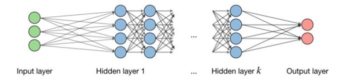
Neural Network Schematic

Layer-Interaction

Figure 7 A schematic of a neural network. On the left we have the input layer consisting of three neurons which reaches the output layer of two neurons on the right through a varying number of hidden layers of four neurons each. All neurons of each adjacent layer are fully connected. [63]

Read more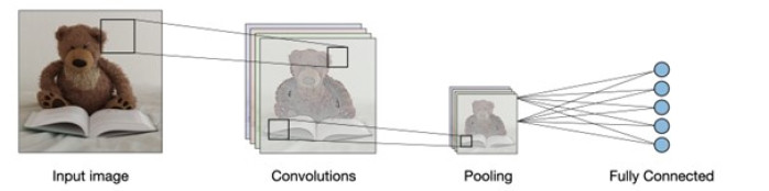

Convolutional Layers

For Image classification

Figure 8 A schematic of a CNN Image classification task. Shown on the left is an image of a Teddy bear as input. A convolution kernel is shown, which relates to the subsequent convolution operations over each color channel. Then a pooling layer is used with a new kernel which stands in relation to the previous input, indicating new image and kernel sizes resulting from downsampling. On the right the model concludes in a fully connected layer of 5 neurons, indicating a classification into 5 classes. [66]

Read more

Materials and Methods

Datasets: PXD005946, PXD005940, Undisclosed Dataset

Dataset Characteristics

The work relies on two PRIDE datasets built around the NCI-60 cell line panel and one internal cohort. The NCI-60 resources provide quantitative proteome and kinome profiles across diverse tissues, quantifying 10,350 proteins, including 375 kinases, with a core cancer proteome of 5,578 proteins consistently observed across tissue types. Samples originate from DTP/NCI cell pellets and were analyzed using kinobead affinity purification in combination with LTQ Orbitrap XL ETD or Orbitrap Elite platforms. These datasets reveal tissue-type clustering, highlight differentially regulated proteins as biomarker candidates, and show concordance between mRNA and protein expression profiles, enabling association of proteome signatures with drug sensitivity and resistance [81, 82].

NCI-60 Datasets

The dataset labeled PXD005946 contains 732 RAW files, a label file, and MaxQuant outputs, acquired on an LTQ Orbitrap XL ETD with a 6,600-second retention window and 300–1,300 m/z range; average RAW size is 217 MB [82]. The dataset labeled PXD005940 comprises 216 RAW files, a label file, and MaxQuant outputs, acquired on an Orbitrap Elite with a 3,600-second retention window and 300–1,300 m/z range; average RAW size is 169 MB [81].

Undisclosed Dataset

The internal cohort is provided as mzML files generated by MSConvert using vendor peakPicking “msLevel1-1” and “msLevel 1-1”. It contains 350 human plasma samples prepared on four 96-well plates by the LMU Protein Analysis Unit, with labels for batch and sex.

Dataset Processing

NCI-60 Datasets

Labels are parsed from the SDRF files to extract classes including sex, organism part (two levels), cell type, and cancer. Labels are stored as nested dictionaries keyed by file name [81, 82]. RAW files are converted with MSConvert to mzML using vendor peakPicking at MS1 where available, OpenMS peakPicking as fallback, zlib compression disabled for custom access, and mzML as the output format. These settings ensure that only precursor-level signals are retained and that downstream parsing remains reliable.

Undisclosed Dataset

Provided labels for sex and plate batch are organized into a dictionary keyed by sample identifiers, mirroring the approach taken for NCI-60.

Original Work

Denoise Algorithms

Two procedures remove signals that systematically confound interpretation at the beginning and end of LC gradients. For the initial isocratic hold, the method scans the first fifth of the run with a moving 100-RT unit window, comparing the medians of left and right halves at each index. When the difference exceeds the current reference by more than 80%, the reference is updated; the rightmost index at which this criterion last holds defines the cutoff. For the high-organic flush, the method analyzes only the final tenth of the run, using a 100-RT unit window centered at each index to track the direction of the local mean intensity. The earliest index of the longest monotonic trend of at least ten consecutive points is returned as the cutoff. These adaptive cutoffs normalize per-run variability in hold and flush behavior without fixed thresholds.

FeatureXML Processing

Two complementary conversions bridge featureXML and mzML to enable targeted learning on feature-level signals. The first conversion extracts retention time, m/z, and intensity for each feature whose RT span is shorter than 50 time units, materializes only those peaks into a new mzML using OpenMS MSSpectrum and MSExperiment, and thereby yields a compact representation of feature centroids. The second conversion identifies the RT and m/z bounding box of each qualifying feature by scanning all points, stores these coordinates, and uses the OpenMS nightly function get2DPeakDataLong to extract all raw signals inside each box from the original mzML before writing a new mzML. The first route preserves concise feature peaks; the second preserves full local signal context for each feature window.

Deep Learning Model

The image-based classifier adapts the TensorFlow image classification template [75] with custom kernels, strides, regularization, and learning rate to suit MS1 patterns. The architecture rescales inputs, applies dropout, stacks three convolutional blocks with max-pooling, flattens, and finishes with a dense hidden layer and a softmax output sized to the number of classes. Convolutions use ReLU with “same” padding; kernels are 3×6 in the first block and 5×5 in later blocks with filter counts of 8, 216, and 64, respectively. The model is trained with categorical cross-entropy and Adam at a learning rate of 1.68×10⁻⁴, and accuracy is tracked during training. This configuration reflects a bias toward moderate capacity and spatial anisotropy in early kernels to better capture RT–m/z structures.

Pseudo code for the CNN (Figure 9)

define NUM_CLASSES from label set
define INPUT_SHAPE as (IMG_HEIGHT, IMG_WIDTH, 3)

initialize MODEL

add Rescaling layer to normalize pixels to [0, 1]
add Dropout layer with rate 0.07

add Conv2D with filters=8, kernel=(3,6), stride=1, padding="same", activation=ReLU
add MaxPooling2D

add Conv2D with filters=216, kernel=(5,5), stride=2, padding="same", activation=ReLU
add MaxPooling2D

add Conv2D with filters=64, kernel=(5,5), stride=2, padding="same", activation=ReLU
add MaxPooling2D

add Flatten

add Dense with units=500, activation=ReLU
add Dense with units=NUM_CLASSES, activation=Softmax

compile MODEL with:
  loss = CategoricalCrossentropy
  optimizer = Adam(learning_rate=0.000168)
  metrics = ["accuracy"]

Figure 9 Architecture of the used Keras deep learning model. The provided code (in this case only as pseudo code for simplicity) defines a convolutional neural network model using the Keras API for a classification task. It includes convolutional layers with different kernel sizes and activation functions, followed by max-pooling layers. Afterward, the data is flattened, and two dense layers, of which one is used for classification in respect to the number of input classes. The model is compiled with categorical cross-entropy as the loss function, Adam optimizer, and accuracy as the evaluation metric.

Blueprint: Feature Alignment

The alignment strategy formalizes anchor points based on biochemical priors and observed features, then applies a star-wise transformation to bring all samples into a common coordinate system. A comprehensive tryptic peptide list with expected precursor ions is generated using Expasy PeptideMass [83] and stored with characteristic metadata. The template sample is chosen as the run with the largest number of signals; its FeatureFinderCentroided output is examined for features that exhibit a consistent ladder of charge states and m/z values corresponding to a single precursor with multiple charges, and these are added to the anchor dictionary. Each target mzML is then scanned to locate these anchors; their RT–m/z coordinates are written into an index. Alignment proceeds by mapping each target to the template (star-wise). Offsets from matched anchors are applied to the target’s coordinates with a gradient-based interpolation for intermediate points that weights distances to adjacent offset vectors and respects any prior per-point offsets. The transformed signals are exported as aligned mzML files, enabling consistent downstream analysis across batches and instruments.

Core Principles

Denoise Algorithms

The first denoising algorithm targets the initial isocratic hold and imitates contour detection to locate the point where the gradient begins ramping up. It applies a moving window and compares the medians of its left and right halves to minimize the impact of random high-intensity spikes. Based on guidance from laboratory technicians and empirical testing on over 200 samples, the algorithm assumes that the isocratic hold typically occurs within the first 20% of the run, and it uses a contrast threshold of 80% as the trigger for detecting the end of this phase.

The second denoising algorithm removes the high-organic flush at the end of LC runs. It applies a centered sliding window of mean values to suppress the impact of sparse zero or low-intensity values on an otherwise monotonous gradient. Based on lab experience, this flush phase is expected to occur within the final 10% of the retention time. The algorithm returns the index where the longest strictly monotonic trend begins, effectively retaining only the preceding signals.

FeatureXML Processing

FeatureXML outputs from the FeatureFinderCentroided tool are repurposed as noise filters to extract only meaningful peaks from the original mzML files. Two complementary algorithms are used: a peak-focused approach that compresses feature windows to their centroid signals for storage efficiency, and a feature-window approach that preserves the original resolution of feature regions. Both approaches remove signals that exceed the expected retention time width of typical peptide features, ensuring consistent input data quality for downstream image creation and learning tasks.

Deep Learning Model

A convolutional neural network (CNN) architecture is selected due to its strength in image pattern recognition. Images are rescaled to reduce the RGB channel intensity range and improve convergence. A dropout rate of 0.07 prevents overfitting without harming learning stability.

The first convolutional layer uses a wide kernel and stride to detect local high-intensity peaks, absorb retention time shifts, and capture m/z deviations of up to one pixel. Subsequent layers use larger, equilateral kernels with larger strides to capture long-range relationships between distant or peripheral signals while improving training speed. All convolutions use 'same' padding to preserve border information, and ReLU is used as the activation function. Max-pooling layers downsample data and emphasize peak values, reducing computational load while preserving salient features.

After convolution, the flatten layer converts spatial feature maps into a one-dimensional vector, which is passed into a dense layer designed with a large number of neurons. This accounts for the estimated maximum number of precursor ions linked to a parent ion, and their complex intensity relationships, tuned using KerasTuner. The final dense layer applies softmax activation for multiclass classification. Categorical crossentropy is used as the loss function, and the Adam optimizer (with its learning rate tuned via KerasTuner) manages weight updates during training.

Blueprint: Feature Alignment

Blood sample alignment

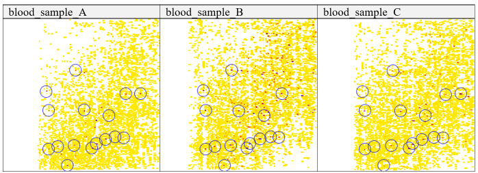
an example of signal variability

Table 2 Blood plasma samples with framed high intensity features. Blue circles frame high intensity signals in three different blood samples in representation of recurring high intensity signal patterns in all blood plasma samples.

Visual inspection of heatmaps from different blood samples revealed recurring high-intensity signal clusters across all samples. These clusters often appeared distorted along the retention time axis but still formed a recognizable pattern, suggesting their origin from specific abundant blood proteins such as albumin or from consistent experimental reagents or labels. Because these precursor ions recur reliably, they are well suited as empirically derived anchor points for alignment.

The alignment blueprint uses these recurring anchors as fixed points. It gradually applies offsets to all in-between signals while referencing the grid-based structure of SOMs (as described in 2.1.2.1). By interpolating between neighboring anchor offsets, the method simulates the inertia of LC flow and corrects local distortions, producing consistently aligned feature maps across different samples.

Implementation

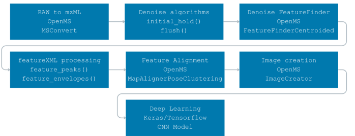
The flow below shows how raw vendor files become model-ready images and how each algorithm fits into that path.

Process of implementation

Each step of my implementation

Figure 10 Flow diagram of all steps involved. The flow diagram illustrates all the steps involved in the implementation process, each labeled with descriptive titles and the corresponding algorithms/tools used. The flow starts at the top left and moves to the left on each line, ending at the bottom.

The RAW-to-mzML conversion follows 3.1.3 using MSConvertGUI. Subsequent OpenMS tasks can be run with TOPPAS defaults (cross-platform instructions are on the OpenMS GitHub [56]).

Denoise algorithms

The dataframe-to-series preparation creates one representative value per retention-time (RT) unit for robust downstream cutoff detection.

Preparation for both cutoff algorithms (pseudo code for Figure 11)

function PREPARE_RT_SERIES(from mzML_dataframe):
  create RT_VALUES mapping each integer RT to default value 1
  for each spectrum in dataframe:
    if spectrum has nonzero intensities:
      RT_KEY ← integer RT of spectrum
      MEAN_INTENSITY ← average of intensities
      LENGTH_OVER_MEAN ← count(intensities) / MEAN_INTENSITY
      RT_VALUES[RT_KEY] ← LENGTH_OVER_MEAN
  return LOG_TRANSFORM(all RT_VALUES in RT order)

Figure 11 Source code to prepare dataframe for cutoff algorithms. The Source code applies required transformations to a mzML dataframe to make data applicable to both lc gradient cutoff algorithms. It calculates the length of an intensity interval divided by the average of intensities and passes it as value to a dictionary for each retention time unit.

Figure 12 — Initial Isocratic Hold cutoff

function FIND_INITIAL_HOLD(y_series, window_size, percent_threshold, base_cutoff_index, search_rt_limit):
  START ← half(window_size) − 1
  END   ← last RT index
  BEST_CONTRAST ← 0
  CUTOFF_INDEX  ← 0

  for index from START to END step 1:
    if y_series[index] ≠ 0:
      LEFT_MEDIAN  ← median(nonzero values in window left of index)
      RIGHT_MEDIAN ← median(nonzero values in window right of index)
      CURRENT_CONTRAST ← |LEFT_MEDIAN − RIGHT_MEDIAN|

      if index ≥ search_rt_limit + window_size:
        if CUTOFF_INDEX = 0: CUTOFF_INDEX ← base_cutoff_index
        break

      else if CURRENT_CONTRAST > BEST_CONTRAST × (1 + percent_threshold):
        CUTOFF_INDEX  ← index
        BEST_CONTRAST ← CURRENT_CONTRAST

  return CUTOFF_INDEX

Figure 12 Source code for the initial isocratic hold cutoff algorithm. Mandatory parameters are a variable including the dictionary acquired dictionary from Figure 11, size of the moving window, threshold for the retention time window as percentage, base cutoff as percentage and the retention time length resulting from the chosen percentage threshold.

Figure 13 — High-Organic Flush cutoff

function FIND_FLUSH_START(y_series, min_consecutive = 10):
  WINDOW_SIZE ← 100 RT units
  REGION ← last 10% of run (indices padded by half window)

  PREV_MEAN ← undefined
  CURRENT_TREND ← none
  CONSECUTIVE_STEPS ← 0
  LONGEST_START ← 0
  LONGEST_LEN   ← 0
  TEMP_START    ← 0

  for index in REGION:
    WINDOW_MEAN ← mean(nonzero values in centered WINDOW_SIZE)

    if PREV_MEAN is defined:
      if WINDOW_MEAN > PREV_MEAN: new_trend ← increasing
      else if WINDOW_MEAN < PREV_MEAN: new_trend ← decreasing
      else: new_trend ← flat

      if new_trend = CURRENT_TREND and new_trend ≠ flat:
        CONSECUTIVE_STEPS ← CONSECUTIVE_STEPS + 1
      else:
        CURRENT_TREND ← new_trend
        CONSECUTIVE_STEPS ← 1
        TEMP_START ← index

      if CONSECUTIVE_STEPS = min_consecutive:
        LONGEST_START ← TEMP_START
        LONGEST_LEN   ← CONSECUTIVE_STEPS
      else if CONSECUTIVE_STEPS > LONGEST_LEN:
        LONGEST_START ← TEMP_START
        LONGEST_LEN   ← CONSECUTIVE_STEPS

    PREV_MEAN ← WINDOW_MEAN

  return LONGEST_START

Figure 13 Source code for the high organic flush cutoff algorithm. Mandatory parameters are a variable including the dictionary acquired dictionary from Figure 11 and an Integer as an accepted minimum of consecutive values to represent a monotonous trend.

FeatureXML Processing

Figures 14–15 — Feature Peaks path

function EXTRACT_FEATURE_PEAKS(featureXML_path):
  FEATURE_PEAKS ← empty
  buffer current feature's RTs, m/zs, intensities

  for each line in featureXML:
    if line starts a new :
      if previous feature exists and RT span ≤ 50:
        store its representative (RT, m/z, intensity) in FEATURE_PEAKS
      reset buffers for new feature
    else if line contains a point/position:
      accumulate RT, m/z, intensity for current feature

  return FEATURE_PEAKS

function WRITE_CENTROID_MZML(FEATURE_PEAKS, output_path, rt_range, mz_range):
  NEW_EXP ← empty experiment
  add empty spectra at (rt_min, mz_min) and (rt_max, mz_max) to preserve dimensions
  for each (RT, m/z, intensity) in FEATURE_PEAKS:
    write a spectrum at RT with one peak (m/z, intensity)
    append to NEW_EXP
  save NEW_EXP as mzML to output_path

Figure 14 Source code of the algorithm to extract peaks from featureXML files. Mandatory parameters are input files path and output path.

Figure 15 Source code for creating mzML file from extracted peaks. The source code follows the corresponding outline in 3.2.1. of mzML file creation from acquired feature peaks. The function is to be initialized before Figure 14.

Figures 16–17 — Feature Windows path

function EXTRACT_FEATURE_WINDOWS(featureXML_path):
  FEATURE_WINDOWS ← empty
  buffer current feature's RT and m/z tracks

  for each line in featureXML:
    if line starts a new :
      if previous feature exists and RT span ≤ 50:
        record bounding box [min_RT, max_RT, min_mz, max_mz] in FEATURE_WINDOWS
      reset buffers for new feature
    else if line contains a point:
      append RT and m/z to buffers

  return FEATURE_WINDOWS

function WRITE_WINDOWED_MZML(FEATURE_WINDOWS, source_mzML_path, output_path, rt_range, mz_range):
  SOURCE_EXP ← load source mzML
  NEW_EXP ← empty experiment
  add empty spectra at (rt_min, mz_min) and (rt_max, mz_max) to preserve dimensions

  for each BOX in FEATURE_WINDOWS:
    extract all peaks within BOX from SOURCE_EXP (2D query)
    group extracted peaks by RT
    for each RT group:
      write spectrum containing all (m/z, intensity) at that RT
      append to NEW_EXP

  save NEW_EXP as mzML to output_path

Figure 16 Source code of the algorithm to extract feature windows from the original mzML file. Mandatory parameters are input files path, output path and path of the original mzML files path.

Figure 17 Source code for creating mzML file from extracted feature windows. The source code follows the corresponding outline in 3.2.1. for feature window extraction and mzML-file creation. The function is to be initialized before Figure 16.

Deep Learning Model

Load Training Dataset

After generating images from the processed mzML files, they are organized into a folder structure according to their class labels. This structure is then used to load the data as tensors using Keras’ image_dataset_from_directory method. An 80/20 train/validation split is applied, and prefetching is enabled to optimize GPU usage during training.

function LOAD_DATASET_FROM_FOLDERS(root_path, img_size=(299,299), batch_size=32, seed):
  SPLIT ← 80% train, 20% validation
  TRAIN_DS ← tensors from subfolders under root_path with inferred categorical labels
  VAL_DS   ← tensors from same tree held out by validation split
  enable PREFETCH on TRAIN_DS and VAL_DS for async loading
  return TRAIN_DS, VAL_DS

Figure 18 Loading dataset from folder structure. Images are loaded as tensors from folder structure, inferring categorical labels from folder names through Keras ‘image_dataset_from_directory’ function. An 80% training 20% validation split is applied, and corresponding variables are assigned. Tensors are saved in batches of size 32, image sizes are conserved from original image dimensions, being of 299x299x3. Subsequently, prefetch is enabled for both splits to preload images of the next iteration during training.

KerasTuner

KerasTuner is used between manual trials to optimize key hyperparameters based on accuracy. Ranges are defined for dropout, filter counts, kernel sizes, strides, dense layer size, and learning rate. A random search strategy is applied to explore the hyperparameter space and return the best model.

function BUILD_MODEL_WITH_HP(hp):
  input ← image tensor (H, W, 3)
  x ← RESCALE pixels to [0,1]
  x ← DROPOUT(rate = hp.float 0.00..0.20 step 0.01)
  x ← CONV(filters = hp.int 8..64 step 8,
           kernel = (hp.choice {3,7}, hp.choice {3,7}),
           stride  = hp.choice {1,4},
           activation = ReLU, padding="same")
  x ← MAXPOOL
  x ← CONV(filters = hp.int 32..256 step 32,
           kernel = (hp.choice {3,7}, hp.choice {3,7}),
           stride  = hp.choice {1,4},
           activation = ReLU, padding="same")
  x ← MAXPOOL
  x ← CONV(filters = hp.int 64..256 step 32,
           kernel = hp.choice {3,10},
           stride  = hp.choice {1,4},
           activation = ReLU, padding="same")
  x ← MAXPOOL
  x ← FLATTEN
  x ← DENSE(units = hp.int 299..700 step 100, activation = ReLU)
  output ← DENSE(units = NUM_CLASSES, activation = Softmax)
  model ← assemble(input, output)
  LR ← hp.float 1e-5..1e-3 (log scale)
  compile(model, optimizer = Adam(LR), loss = CategoricalCrossentropy, metrics = ["accuracy"])
  return model

procedure RUN_TUNER(train_ds, val_ds):
  tuner ← RandomSearch(build_fn = BUILD_MODEL_WITH_HP,
                       objective = "val_loss",
                       max_trials = 100,
                       executions_per_trial = 3,
                       workdir = "output_tuner",
                       overwrite = true)
  tuner.search(train_ds, epochs = 100, validation_data = val_ds,
               callbacks = [TensorBoard for tuner])
  best_model ← tuner.best_models[0]
  return best_model

Figure 19 Source code for KerasTuner build into the models Architecture. For every hyperparameter of interest the ‘hp’ argument is introduced and corresponding functions Choice(), Int() and Float() are applied. Ranges of variation are randomly centered around the models initialization values to monitor their performance.

Deep Learning Model Setup

Based on the selected architecture from the design phase, the CNN model is constructed using convolutional, pooling, and dense layers. It uses ReLU activations and a softmax output layer. The model is then compiled with categorical crossentropy loss and the Adam optimizer.

function BUILD_BASE_MODEL(img_size=(299,299), num_classes):
  input ← image tensor (H, W, 3)
  x ← RESCALE to [0,1]
  x ← DROPOUT(rate = 0.07)
  x ← CONV(filters=8,   kernel=(3,6), stride=1, activation=ReLU, padding="same")
  x ← MAXPOOL
  x ← CONV(filters=216, kernel=(5,5), stride=2, activation=ReLU, padding="same")
  x ← MAXPOOL
  x ← CONV(filters=64,  kernel=(5,5), stride=2, activation=ReLU, padding="same")
  x ← MAXPOOL
  x ← FLATTEN
  x ← DENSE(units=500, activation=ReLU)
  output ← DENSE(units=num_classes, activation=Softmax)
  model ← assemble(input, output)
  return model

procedure COMPILE_MODEL(model):
  LOSS ← CategoricalCrossentropy
  OPT  ← Adam(learning_rate = 0.000168)
  METRICS ← ["accuracy"]
  compile(model, optimizer = OPT, loss = LOSS, metrics = METRICS)
  return model

Figure 20 Build of the deep learning model. The model is constructed based on the provided source code, as explained in section 3.2.3

Figure 21 Compilation of the deep learning model. As stated in section 3.2.3, the model uses categorical crossentropy as the loss function for handling multiclass classification, where each class is represented by a one-hot binary array. The optimizer chosen is 'Adam', with a learning rate set to 0.000168. The accuracy metric is tracked during training.

Training

The compiled model is trained on the training dataset for 150 epochs with validation on the held-out set. Early stopping, checkpoint saving, and TensorBoard logging callbacks are enabled to monitor and manage training progress.

function TRAIN_MODEL(model, train_ds, val_ds, epochs=150):
  CALLBACKS ← [EarlyStopping(on validation loss), ModelCheckpoint(save best),
               TensorBoard(logging)]
  HISTORY ← fit(model, train_ds,
                validation_data = val_ds,
                epochs = epochs,
                callbacks = CALLBACKS)
  return HISTORY

Figure 22 Fitting of the deep learning model. The model is trained for 150 epochs using dataset splits from section 3.4.4.1. Callbacks are implemented to perform early stopping if the generalization error stops decreasing. Model checkpoints are used to save the weights at each learning step, and TensorBoard is employed to access the TensorBoard user interface for visualization and analysis.

Prediction and Evaluation

Predictions are made on the processed files of the PXD005940 dataset using the Keras predict() method.
For evaluation, Keras stand-alone metrics for Precision, Recall, and Accuracy are used to assess model performance.

Processing Unit

Data processing and model training were carried out on an AMD system running Windows 11 Pro (22H2).
The system specifications are:

Processor: AMD Ryzen 7 3800X @ 3.90 GHz
RAM: 32 GB 3200 MHz
GPU: Radeon RX 6800 (16 GB VRAM)

IDE, Python and Libraries

All implementations were written in Python 3.9 using PyCharm and Visual Studio Code (VS Code) as integrated development environments (IDEs).
Dependencies correspond to their most current releases as of 03/2023, except for pyopenms, which required the pre-nightly build OpenMS-3.0.0-pre-nightly-2022-11-17.

General compatibility relied on the availability of two OpenMS functions — get2DPeakDataLong and get_df — which were not present in the official release build during the time of this thesis.

Availability

The NCI-60 datasets are publicly available via PRIDE (PXD005940 and PXD005946).
The undisclosed dataset is internal and not publicly accessible.

Results and Discussion

mzML-Preprocessing

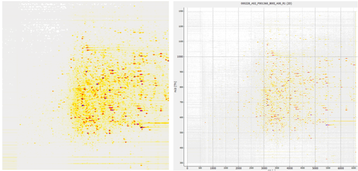
As a starting point for the mzML conversion of the acquired RAW files, spectra with the dimensions of 6600 seconds as retention timeframe and 300-1300 m/z values are obtained according to the specifications of the Dataset PXD005946. Figure 23 shows how such unprocessed data looks before various denoising and transformation operations are applied.

mzML as image

by OpenMS ImageCreator

Figure 23 mzML-file image representation. Both images represent the sample 000228_A02_P001360_B00I_A00_R1 in the PXD005946 dataset. The image on the left was processed by OpenMS ImageCreator with output dimensions 299x299x3. On the right is the visual representation in OpenMS TOPPView for all datapoints included.

While not inherently clear from the previous example why data may need further denoise, Figure 24 clarifies what variances can be expected.

encountered variances

through various classes

Figure 24 Images of an earlier classification task involving the Dataset PXD005946. The previous classification task involved 45 selected disease classes in their various types of occurrences, encoded as integers. Title of each image refers to a specific class. Both images to the left show an overall normal spectrum, while images to the right involve multiple distortions and prominent high intensity peculiarities.

Overly long distorted signals and non-signal related artefacts confused the convolutional neural network, hindering the training success and often leading to overfitting, as the model shifted its attention from complex signal patterns to more convolutionally prevalent peculiarities. The data-preprocessing step offers versatility in handling various conversion options using OpenMS tools, accommodating a wide range of file formats, including initially unsupported formats like multiplexed data. Utilizing Pandas dataframes, the OpenMS nightly build's get_df function, and custom scripts with subsequent use of OpenMS mzML handlers, offers a starting point on how to extract essential data such as intensity, separation time, m/z, and optional information like the LC gradient events from manufacturer-specific file formats.

RAW to mzML Conversion

File conversion without compression applied led to increased file sizes for resulting mzML files. Average file sizes before and after the conversion process are shown in Table 3.

raw_to_mzML	Average file sizes: after	Average file sizes: before
PXD005946	315 MB ↑	217 MB
PXD005940	341 MB ↑	169 MB

Table 3 Observed average file-size changes during RAW to mzML conversion. After-values are provided with an indicator, stating the size change direction in comparison to before file conversion. A red upward arrow indicates an undesired increase in file size for both NCl-60 Datasets.

mzML-Trimming: LC Gradient Profile Cutoffs

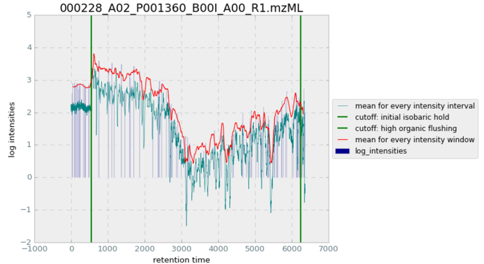
The two cutoff algorithms for the LC gradient yield multiple values that can be tracked and visualized in Figure 25. The mean for every intensity interval is taken from the intensity arrays associated with every retention time value. The mean for every intensity window is monitored with the running window being applied to the whole experiment run.

cutoff visualisation

shown on the spectra

Figure 25 Diagram of mzML-trimming cutoffs and for PXD005946 000228_A02_P001360_B00I_A00_R1 for running-window evaluation and overall signal distributions. Green vertical bars display where both algorithms returned their cutoff value, showing their success on tracing contrast and monotonous trend, as well as the general suitability of tracked values to derive corresponding expressiveness.

While the exact position of applied cutoffs showed to need more fine-tuning, both algorithms generalized surprisingly well on the majority of samples, reliably applying dynamic cutoffs in near proximity of desired thresholds. Figure 26 and Table 4 show how cutoffs apply to the now initially processed data before alignment and FeatureFinder are applied.

cutoff visualisation

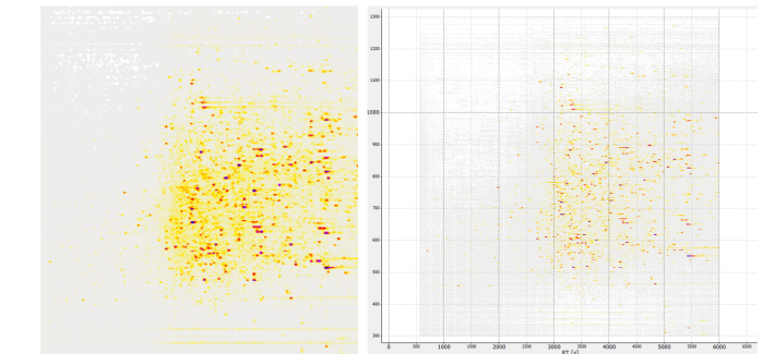
shown on 2D image

Figure 26 mzML-file image representation after mzML-trimming for PXD005946 000228_A02_P001360_B00I_A00_R1. Left: OpenMS ImageCreator 299x299x3. Right: openMS TOPView

lc_cutoffs	Average file sizes: after	Average file sizes: before
PXD005946	187 MB ↓	315 MB
PXD005940	164 MB ↓	341 MB

Table 4 Observed average file-size changes during mzML-trimming. A green downward arrow indicates a desired decrease in file size for both NCl-60 Datasets.

Resulting from the use of a similar version of the mzML-converter introduced in 3.4.1.1 for refeeding the remainder after cutoffs to a new mzML file, the decrease of file size cannot be attributed to the trimming step. Whilst being applied over all signals of the original mzML file, any secondary information is not preserved. This results in a significant decrease of file size instead of the anticipated small margin through applied cutoffs for up to 30 % of the data at maximum.

mzML-Alignment

mzML-Alignment was skipped for the NCI-60 datasets due to versatility of classes and tissue-specific biochemical variety. Figure 27 shows an example from the undisclosed human blood sample dataset, aligning two samples:

mzML-Alignment

for signals of interest

Figure 27 Map alignment example. The illustrated feature maps represent only the 99th percentile of each intensity mean for signal coordinates. Left: Two feature maps with different retention time and mass-to-charge dimensions. Right: The features of the second feature maps were transformed onto the coordinate system of the first feature map.

As not directly visible, the accompanied .trafo file often has to be consulted to see what alignments were made.

Feature Extraction: feature_envelopes, feature_peaks

Figure 28 shows how FeatureFinderCentroided is applied to original mzML files, framing isotopic envelopes of varying dimensions and intensities. Table 5 lists the resulting file sizes after both signal extraction operations (feature_envelopes and feature_peaks as described in 3.4.2).

feature windows

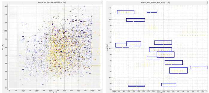
scattering of signals

Figure 28 featureXML-file image representation after OpenMS FeatureFinderCentroided for PXD005946 000228_A02_P001360_B00I_A00_R1, showing feature envelopes superimposed on the original mzML file. Left: openMS TOPView for whole spectrum. Right: openMS TOPView for rt: 3200-3390 and m/z: 896-925 segment

feature_envelopes, feature_peaks	Average file sizes: after	Average file sizes: before
PXD005946	88 MB ↓ , 12 MB ↓	187 MB
PXD005940	168 MB ↑ , 10 MB ↓	164 MB

Table 5 Observed average file-size changes for FeatureFinderCentroided outputs after conversion to mzML for feature envelopes (feature_envelopes) and centroid peaks (feature_peaks). Files created from FeatureFinderCentroided show a significant decrease of file-size if only extracted peaks are included. If feature windows were extracted from original mzML files, a significant decrease could only be observed for PXD005946, while file-sizes for PXD005940 slightly increased.

Image Creation

Images were created in different resolutions, feature representations, with and without log transformations applied on the intensity gradients. Tables 6–9 summarize the results.

different resolutions

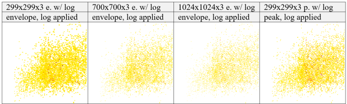
with log applied

Table 6 PXD005946: 000228_A02_P001360_B00I_A00_R1 Image representations. Images represent each abstraction level after Image creation step for dimensions of 299x299x3, 700x700x3, 1024x1024x3 on feature_envelopes and 299x299x3 on feature_peaks, with log transformation applied on intensity gradients, left to right.

different resolutions

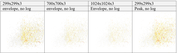
without log applied

Table 7 Image representations without log applied. Images represent each abstraction level after Image creation step for dimensions of 299x299x3, 700x700x3, 1024x1024x3 on feature_envelopes and 299x299x3 on feature_peaks, without log transformation applied, left to right.

feature_envelopes	Image sizes	Log gradient	After: avg. filesize	Before: avg. filesize
PXD005946	299x299 / 700x700 / 1024x1024	True, False	37 KB–138 KB ↓	88 MB, 12 MB
PXD005940	299x299 / 700x700 / 1024x1024	True, False	35 KB–134 KB ↓	168 MB, 10 MB

Table 8 Observed average file-size changes. Monitored was the image creation on feature_envelopes with dimensions of 299x299x3, 700x700x3, 1024x1024x3 with Boolean values for applying log to intensity gradients for both NCl-60 datasets.

feature_peaks	Image sizes	Log gradient	After	Before
PXD005946	299x299	True, False	40 KB ↓, 63 KB ↓	88 MB, 12 MB
PXD005940	299x299	True, False	32 KB ↓, 51 KB ↓	168 MB, 10 MB

Table 9 Observed average file-size changes. Monitored was the image creation on feature_peaks with dimensions of 299x299x3 with Boolean values for applying log to intensity gradients for both NCl-60 datasets.

Goal was to feed different image sizes to the model and assess the most suitable format for training success. In respect to the progress made on the 299x299 images, no further benchmarks were made for the set classification task of 9 common [bodypart, tissue] labels.

Deep Learning

KerasTuner Performance

KerasTuner, as displayed in Table 10, benchmarked and improved passed hyperparameter ranges over 30 trial runs with 3 executions per trial over 150 epochs, resulting in the best validation accuracy of 0.62 with a validation loss of 1.58 whilst being able to reliably learn the complexity of the training set.

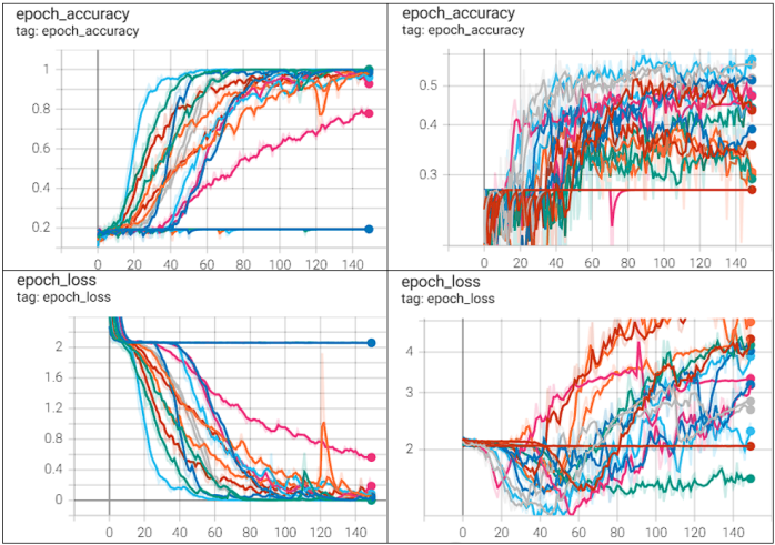
models epoch performance

with KerasTuner

Table 10 TensorBoard visualization of performances of KerasTuner automated hyperparameter tuning over 30 trial runs with 150 epochs, accuracy/loss on the y-axis, epochs on the x-axis. Left: epoch-accuracy (top) and epoch-loss (bottom) for training. Right: epoch-accuracy (top) and epoch-loss (bottom) for validation.

Hyperparameter tuning of the model was perceived as a trade-off between applying comprehensively acclaimed settings and trial-and-error.
Offside the basic hyperparameters there is a vast variety of mathematical functions to account for different aspects of the model and processed data. The Keras API reference [67] alone lists 10 standard functions for probabilistic losses [84], 9 standard layer activation functions [64] and 10 standard optimizers [70], without considering custom approaches and parameters within each function.

Although being of specific classification nature — for example “Binary_Crossentropy” with “sigmoid” being specific for binary classification approaches and “Categorical_Crossentropy” with “softmax” activation for multiclass classification — the sheer extent of possible combinations became too time consuming.

In respect to the time constraints and scope of this bachelor's thesis, it became clear after testing through trial and error that the basic tutorial hyperparameters with their default settings would suffice for this project.
Notably the optimizer’s learning rate parameter remains a crucial tuning lever, as it determines the degree of emphasis placed on weight updates during model training.

Model Results

For the resulting model with transferred values from KerasTuner and further adjustments through trial-and-error, the model training performance is shown in Figure 29, tracking training and validation accuracy on the left side and training and validation loss on the right side.

An early stop was applied at 72 epochs, as validation loss did not further decrease after a patience span of 30 epochs, marking epoch 43 as its peak (validation loss = 1.3573, validation accuracy = 0.3913).

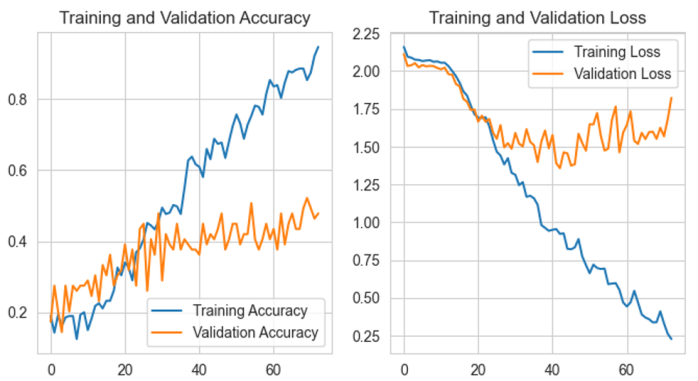
Model performance

final model

Figure 29 Accuracy and validation visualization, x-axis shows [accuracy, loss] values, y-axis shows epochs for a selected run. Left: Training and Validation Accuracy. Right: Training and Validation Loss.

The accuracy diagram shows that the validation process cannot surpass a projected border at around 0.52, while the model is able to converge on the training set to reliable classification.
The validation loss diagram shows a projected border at 1.3573 validation loss, which then increases up to 1.6814, converging back to its initial validation loss of 2.1119.

This indicates that the model is overfitting to the training data, performing well on the training set but struggling to generalize to the validation set.

As KerasTuner was also not able to yield better performances, multiple assumptions can be made:
The dataset may be imbalanced (9 classes include the following sample counts: [12, 24, 36, 12, 36, 59, 73, 60, 36]); the model might be too shallow; or chosen hyperparameters still not optimal given that KerasTuner only ran for around 24 hours.

Model Predictions

For prediction on the unseen PXD005940 dataset (almost equal class sizes: [24,…,24,21]), the Keras predict() method did not yield any values greater than 0.1 for any metric.
In light of the identified problems, this is not surprising — nevertheless, the predictions were further analyzed.

Figure 30 shows an initial assessment of overall signal contribution between the predicted class and original file:

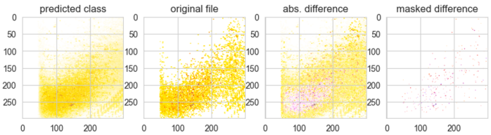
Predictions

highlighting features

Figure 30 Predicted class for one evaluated sample. Images show, from left to right, all images over one class superimposed with a proportional opacity. The second images show the original file used during the prediction. The third image shows the difference between the predicted class stacked signals and original file signals, highlighting highest intensity peaks standing out from the predicted class. The last image shows the highest intensity peak without the overlay of the predicted class.

Saliency maps for each class over each convolutional layer were then created (Figure 31):

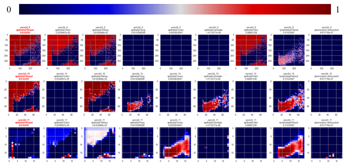
feature importance

for each layer

Figure 31 Saliency maps for class prediction. The top gradient shows the applied weights, dark blue relates to the background of 0 weight, while dark red denotes for high weighted attributes. Every line of the plot accounts for one of three successive convolutional layers within the model. The predicted class is highlighted, by a red image title. The title of each image includes the name of the convolutional layer, associated class, and prediction value.

Looking at the bottom left image at segment position (0, 2), a continuous vertical shape is being highlighted in the first column of image segments.
As it lies near the initial isocratic hold cutoff and exhibits a continuous shape covering multiple image segments, this is interpreted as the model learning convolutionally prevalent peculiarities, supporting the overfitting conclusion.

Figure 32 shows random examples of class images:

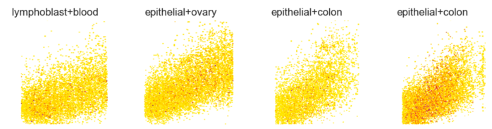
feature differences

on random selected class images

Figure 32 A random selection of class images. Four images are randomly selected to represent four different classes. Image titles refer to the assigned class used during supervised learning.

The signals strongly overlap, and individual signals (except for high-intensity peaks) are difficult to identify.
This shows that at 299x299 resolution, individual features are not separable, which prevents accurate class assignment — although the data shows enough complexity to potentially capture relational dependencies.

This is further supported by Figure 33, which shows saliency maps from a previous classification task of 45 classes (also PXD005946), trained at 299x299x3 input size without LC gradient cutoffs:

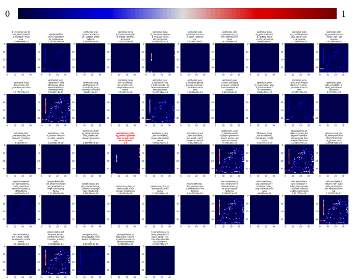
feature importance

for 45 classes in PXD005946

Figure 33 Saliency maps for a previous classification task of 45 classes in PXD005946. The top gradient shows the applied weights, dark blue relates to the background of 0 weight, while dark red denotes for high weighted attributes. All images account for the last convolutional layer in three successive convolutional layers within the model. The predicted class is highlighted, by a red image title. The title of each image includes the associated class, and prediction value.

That model trained successfully (early stopping after 74 epochs, training loss 1.8896e-06, training accuracy 1.0000, validation loss 0.0850, validation accuracy 0.9926).
However, it was not further fine-tuned, as noise factors could not be invalidated and the large number of classes rendered it incompatible with other datasets.

Dataset Size and Augmentation

Another PRIDE dataset (PXD013455) showed potential but only contained multiplex .wiff data, requiring a complex pipeline not feasible within the timeframe.

Dataset size was also limiting: reliable training usually needs ~10× as many samples as classes, but PXD005946 had only ~200 samples across 49 sub-classes, with some classes having fewer than 3 samples.

Augmentation was tested as a possible mitigation using a simple Keras approach (Figure 34):

data_augmentation = tf.keras.Sequential([
    tf.keras.layers.RandomTranslation(
        height_factor=0,
        width_factor=0.01,
        fill_mode="constant",
        fill_value=255),
    tf.keras.layers.RandomZoom(
        height_factor=0,
        width_factor=0.003,
        interpolation="nearest",
        fill_mode="constant",
        fill_value=255),
    tf.keras.layers.Rescaling(1./255)
])

Figure 34 Source for a tested file Augmentation. The Augmentation aims to apply artificial distortion similar to retention time offsets experienced between samples.

This aimed to simulate retention time offsets and width distortions of ±10 pixels, filling empty areas with white (255). However, augmentation was later disabled, as the project focus shifted from convolutional learned signal relations to traceable pattern recognition of naturally occurring signal deviations.

Conclusion and Outlook

During this bachelor’s thesis, a deep learning model was developed that can reliably detect and classify visual patterns in mass spectrometry image data. While the model successfully identified anomalies and peculiarities, time constraints and limited dataset availability prevented full optimization toward consistently recognizing true biochemical features and their underlying structures. The primary bottleneck was the suitability and size of the available datasets, which restricted the model’s ability to generalize and learn complex feature relationships.

Alongside the model, two denoising algorithm sets were implemented to remove systematic LC gradient artifacts—the initial isocratic hold and the high-organic flush. These approaches showed robust performance, though the LC gradient cutoff algorithms exhibited slight deviations from ideal solutions, when compared to manually selected ground-truth values. This deviation largely stemmed from variability among sample types and sample-specific peculiarities, which made creating a universally precise method challenging.

Additionally, a conceptual blueprint was created for a feature alignment algorithm. This approach promises the ability to frame highly sample-specific dominant features within a selected template and to align other samples against this reference in a star-wise fashion, potentially enabling robust cross-run comparison and feature matching.

Looking ahead, future work should focus on acquiring or generating a dataset that meets the model’s requirements in size, consistency, and annotation quality. This would allow for more systematic parameter tuning and architectural experimentation, enabling the model to classify true features and assign them reliably to classes.

The denoising steps could be further refined—particularly the initial FeatureFinderCentroided-based filtering—by optimizing the parameters.ini configuration to better capture meaningful features while excluding low-intensity noise. Similarly, the LC gradient cutoff detection could be enhanced with automated parameter tuning and more sophisticated contour and monotonic behavior analysis to precisely locate transition points.

Moreover, attention should be given to optimizing image dimensions and channel usage. Increasing resolution until feature boundaries lie adjacent without overlap would maximize entropy, while grayscale images might suffice to represent intensity, removing the need for RGB channels. Given that the current model achieves runtimes of only two to fifteen minutes for 299×299×3 images over 150 epochs—and each KerasTuner trial completes within two hours on the described personal system—larger image dimensions and more complex models appear feasible, especially on a GPU-enabled system with CUDA support.

These steps would significantly advance the system toward its goal: reliably identifying true proteomic features, classifying them, and enabling robust downstream biological interpretation.

Bibliography

Hoffmann, E.d. and V. Stroobant, Mass spectrometry: principles and applications. 3rd ed. 2007, Chichester, West Sussex, England ; Hoboken, NJ: J. Wiley. xii, 489 p.
al., Z.e., Phenotype Prediction using a Tensor Representation and Deep Learning from Data Independent Acquisition Mass Spectrometry. 2020.
GmbH, P.P., Stochos. 2023.
Wang, S., et al., MSpectraAI: a powerful platform for deciphering proteome profiling of multi-tumor mass spectrometry data by using deep neural networks. BMC Bioinformatics, 2020. 21(1): p. 439.
Cadow, J., et al., On the feasibility of deep learning applications using raw mass spectrometry data. Bioinformatics, 2021. 37(Suppl_1): p. i245-i253.
A. Holzinger, P.K., A. Tjoa, E. Weippl (Eds.), Deep Learning for Proteomics Data for Feature Selection and Classification, in Machine Learning and Knowledge extraction, T.C. Sahar Iravani, Editor. 2019.
Iravani, S. and T.O.F. Conrad, An Interpretable Deep Learning Approach for Biomarker Detection in LC-MS Proteomics Data. IEEE/ACM Trans Comput Biol Bioinform, 2023. 20(1): p. 151-161.
fchollet. Image classification from scratch. 2022; Available from: https://keras.io/examples/vision/image_classification_from_scratch/.
Boedecker, D.J. Self-Organizing Map (SOM). Machine Learning 2015; Available from: https://ml.informatik.uni-freiburg.de/former/_media/documents/teaching/ss15/som.pdf.
Kohonen, T., The self-organizing map. Proceedings of the IEEE, 1990. 78: p. 1464-1480.
Giorgino, T., Computing and Visualizing Dynamic Time Warping Alignments in R: The dtw Package. Journal of Statistical Software, 2009.
Lin, A., et al., MS1Connect: a mass spectrometry run similarity measure. Bioinformatics, 2023. 39(2).
Weisser, H., et al., An automated pipeline for high-throughput label-free quantitative proteomics. J Proteome Res, 2013. 12(4): p. 1628-44.
Keras. Code examples. Available from: https://keras.io/examples/.
Springenberg, J.T., Dosovitskiy, A., Brox, T., Riedmiller, M., Striving for simplicity: the all convolutional net. 2014.
C-nit. mass_spec_trans_coding. [cited 2023 12.07.2023]; MSTranc]. Available from: https://github.com/PhosphorylatedRabbits/mass_spec_trans_coding.
wangshisheng. MSpectraAI. [cited 2023 12.07.2023]; MSpectraAI]. Available from: https://github.com/wangshisheng/MSpectraAI.
Keras. ZeroPadding2D layer. Available from: https://keras.io/api/layers/reshaping_layers/zero_padding2d/.
Keiron O'Shea, R.N., An Introduction to Convolutional Neural Networks. 2015.
Giorgino, T. dtw-python. 2022; Available from: https://pypi.org/project/dtw-python/.
bmx8177. MS1Connect. Available from: https://github.com/bmx8177/MS1Connect/tree/main/bin.
OpenMS. MapAlignmentAlgorithmPoseClustering Class Reference. Available from: https://openms.de/doxygen/nightly/html/classOpenMS_1_1MapAlignmentAlgorithmPoseClustering.html.
Lange, E., et al., A geometric approach for the alignment of liquid chromatography-mass spectrometry data. Bioinformatics, 2007. 23(13): p. i273-81.
OpenMS. TransformationDescription Class Reference. Available from: https://openms.de/current_doxygen/html/classOpenMS_1_1TransformationDescription.html.
Team, O. OpenMS Community. Available from: https://openms.de/communication/.
Jarosch, B., Pocket Guide Biologie - ergänzend zum Purves. 2018: Springer Spektrum Berlin, Heidelberg.
Clark, D.P., N.J. Pazdernik, and M.R. McGehee, Molecular biology. Third edition. ed. 2019, London, United Kingdom: Academic Press, an imprint of Elsevier. xv, 1001 pages.
Ankit Sinha, M.M., A beginner’s guide to mass spectrometry–based proteomics. The Biochemist, 2020.
Göttingen, G.-A.-U. Transfusionsmedizin. Vorlesungsbegleitendes Skript 2018; Available from: https://transfusionsmedizin.umg.eu/fileadmin/Redaktion/Transfusionsmedizin/Dokumente/skript_tfm_1_.pdf.
Simpson, R.J. and D.W. Greening, Serum/plasma proteomics: methods and protocols. Second edition. ed. Methods in molecular biology, 2017, New York, NY: Humana Press. xvi, 551 pages.
Scientific, T. Protein Sample Preparation for Mass Spectrometry. Available from: https://www.thermofisher.com/de/de/home/life-science/protein-biology/protein-biology-learning-center/protein-biology-resource-library/pierce-protein-methods/sample-preparation-mass-spectrometry.html.
Keerthikumar, S. and S. Mathivanan, Proteome bioinformatics. Methods in molecular biology, 2017, New York: Humana Press. xi, 233 pages.
Rodriguez J, G.N., Smith RD, Pevzner PA, Does trypsin cut before proline? 2008.
Siepen, J.A., et al., Prediction of missed cleavage sites in tryptic peptides aids protein identification in proteomics. J Proteome Res, 2007. 6(1): p. 399-408.
Shuken, S.R., An Introduction to Mass Spectrometry-Based Proteomics. Journal of Proteome Research, 2023.
Fuerstenau, S.D., et al., Mass Spectrometry of an Intact Virus. Angew Chem Int Ed Engl, 2001. 40(3): p. 541-544.
Lima, N.M., et al., Mass spectrometry applied to diagnosis, prognosis, and therapeutic targets identification for the novel coronavirus SARS-CoV-2: A review. Anal Chim Acta, 2022. 1195: p. 339385.
al., R.e. COVID-19 Mass Spectrometry Coalition. Available from: https://www.manchester.ac.uk/coronavirus-response/science-engineering-coronavirus-projects/mass-spectrometry-coalition/.
Charles E. Mortimer, U.M., Johannes Beck, Chemie: das Basiswissen der Chemie. Vol. 12. 2015: Georg Thieme Verlag. 709.
scientific, c. ESI-MS Peptide Interpretation Guide. Available from: https://cpcscientific.com/esi-ms-peptide-interpretation-guide/.
Smith, R., J.T. Prince, and D. Ventura, A coherent mathematical characterization of isotope trace extraction, isotopic envelope extraction, and LC-MS correspondence. BMC Bioinformatics, 2015. 16 Suppl 7(Suppl 7): p. S1.
Scientific, T.F. Common Background Contamination Ions in Mass Spectrometry. Available from: https://beta-static.fishersci.ca/content/dam/fishersci/en_US/documents/programs/scientific/brochures-and-catalogs/posters/fisher-chemical-poster.pdf.
ThermoFisher. Hochleistungsflüssigchromatographie. Available from: https://www.thermofisher.com/de/de/home/industrial/chromatography/liquid-chromatography-lc.html.
Technologies, A. The LC Handbook. Guide to LC Columns and Method Development; Available from: https://www.agilent.com/cs/library/primers/Public/LC-Handbook-Complete-2.pdf.
Río, A.O.a.A.B.a.P.G.a.M.C.A.a.I.P.a.A.G.-L.a.J.A.D., Citrus paradisi and Citrus sinensis flavonoids: Their influence in the defence mechanism against Penicillium digitatum. Food Chemistry, 2006. 98: p. 351-358.
Banerjee, S. and S. Mazumdar, Electrospray ionization mass spectrometry: a technique to access the information beyond the molecular weight of the analyte. Int J Anal Chem, 2012. 2012: p. 282574.
Shannon Eliuk, A.M., Evolution of Orbitrap Mass Spectrometry Instrumentation.
Savaryn, J.a.T., Timothy and Kelleher, Neil, A researcher's guide to mass spectrometry‐based proteomics. PROTEOMICS, 2016. 16.
Technologies, A. MassHunter Software for Advanced Mass Spectrometry Applications. Available from: https://www.agilent.com/en/product/software-informatics/mass-spectrometry-software.
Scientific, T. Xcalibur Software. Available from: https://www.thermofisher.com/order/catalog/product/de/de/OPTON-30965.
Marsh, A.N., et al., Skyline Batch: An Intuitive User Interface for Batch Processing with Skyline. J Proteome Res, 2022. 21(1): p. 289-294.
Cox, J. and M. Mann, MaxQuant enables high peptide identification rates, individualized p.p.b.-range mass accuracies and proteome-wide protein quantification. Nat Biotechnol, 2008. 26(12): p. 1367-72.
Sturm, M., Bertsch, A., Gröpl, C. et al., OpenMS – An open-source software framework for mass spectrometry. BMC Bioinformatics, 2008. 9.
Team, O. OpenMS User Tutorial. Available from: https://openms.readthedocs.io/en/latest/tutorials-and-quickstart-guides/openms-user-tutorial.html.
Hulstaert, N., et al., ThermoRawFileParser: Modular, Scalable, and Cross-Platform RAW File Conversion. J Proteome Res, 2020. 19(1): p. 537-542.
Timo Sachsenberg, J.P., Chris Bielow. OpenMS. Available from: https://github.com/OpenMS/OpenMS.
Deutsch, E.W., Mass spectrometer output file format mzML. Methods Mol Biol, 2010. 604: p. 319-31.
Keras. Keras layers API. Available from: https://keras.io/api/layers/.
Knoche, M. Super-Resolution. 2017; Available from: https://wiki.tum.de/display/lfdv/Super-Resolution.
OpenMS. TOPPAS. Available from: https://abibuilder.cs.uni-tuebingen.de/archive/openms/Documentation/nightly/html/TOPP_TOPPAS.html.
Wankar, S.a.B.M.a.P., Research Paper on Basic of Artificial Neural Network. 2014. 1(1).
Afshine Amidi, S.A. CS 230 ― Deep Learning. Available from: https://stanford.edu/~shervine/teaching/cs-230/.
Afshine Amidi, S.A. CS 229 - Machine Learning. Available from: https://stanford.edu/~shervine/teaching/cs-229/cheatsheet-deep-learning.
Keras. Layer activation functions. Available from: https://keras.io/api/layers/activations/.
Dai, P. Introduction to Deep Learning (I2DL) (IN2346). 2022; Lecture Slides: Available from: https://dvl.in.tum.de/teaching/i2dl-ss22/.
Afshine Amidi, S.A. Convolutional Neural Networks cheatsheet. CS 230 - Deep Learning; Available from: https://stanford.edu/~shervine/teaching/cs-230/cheatsheet-convolutional-neural-networks.
Keras. Keras API reference. Available from: https://keras.io/api/.
TensorFlow. TensorFlow API Documentation. Available from: https://www.tensorflow.org/api_docs.
Keras. Probabilistic losses. Available from: https://keras.io/api/losses/probabilistic_losses/.
Keras. Optimizers. Available from: https://keras.io/api/optimizers/.
Diederik P. Kingma, J.B., Adam: A Method for Stochastic Optimization. 2017.
Keras. Model training APIs. Available from: https://keras.io/api/models/model_training_apis/.
Keras. Dropout layer. Available from: https://keras.io/api/layers/regularization_layers/dropout/.
Keras. Flatten layer. Available from: https://keras.io/api/layers/reshaping_layers/flatten/.
TensorFlow. Image classification. 2023; Available from: https://www.tensorflow.org/tutorials/images/classification.
Jifeng Dai, H.Q., Yuwen Xiong, Yi Li, Guodong Zhang, Han Hu, Yichen Wei, Deformable Convolutional Networks.
Liqiang Xiao, H.Z., Wenqing Chen, Yongkun Wang, Yaohui Jin, Transformable Convolutional Neural Network for Text Classification. International Joint Conference on Artificial Intelligence (IJCAI), 2018.
Raza, A. Type of convolutions: Deformable and Transformable Convolution. 2019; Available from: https://towardsdatascience.com/type-of-convolutions-deformable-and-transformable-convolution-1f660571eb91.
Keras. Base RNN layer. Available from: https://keras.io/api/layers/recurrent_layers/rnn/.
Karen Simonyan, A.V., Andrew Zisserman, Deep Inside Convolutional Networks: Visualising Image Classification Models and Saliency Maps. 2013.
Martin Frejno, D.B.K., Global Proteome Analysis of the NCI-60 Cell Line Panel. 2017.
Martin Frejno, D.B.K., Global Proteome Analysis of the NCI-60 Cell Line Panel, part 3. 2017.
Expasy. PeptideMass. Available from: https://web.expasy.org/peptide_mass/.
Keras. Losses. Available from: https://keras.io/api/losses/.
Berlin, F. Tutorial Week SWP 2012. Softwarepraktikum Bioinformatik 2012; Available from: http://www.mi.fu-berlin.de/wiki/pub/ABI/PMSB_OpenMS_2012/SWP2012.pdf.